What a solver router actually does
A solver router is not a navigation app. It is a mathematical optimization engine that determines the most efficient way to move goods across a network by balancing multiple competing constraints. While basic pathfinding identifies a single route from point A to point B, a solver router calculates the best combination of routes, schedules, and vehicle assignments for an entire fleet simultaneously.
The distinction matters for last-mile logistics. Simple pathfinding might find the shortest distance, but it ignores critical operational realities like delivery windows, vehicle load capacity, driver hours, or traffic patterns. A solver router treats these as hard or soft constraints within a complex equation. It evaluates millions of potential combinations to minimize total cost while ensuring service level agreements are met.
This process relies on operations research techniques, such as those found in Google’s OR-Tools, which allow developers to define specific search limits and solution strategies. The solver doesn't just guess; it systematically explores the solution space to find an optimal or near-optimal result that a human dispatcher could never calculate manually.
By integrating these constraints, the router reduces empty miles, prevents overloading, and ensures drivers arrive within acceptable time windows. This precision is what drives down last-mile costs, turning logistical chaos into a predictable, efficient operation.
Why static routes fail modern fleets
Traditional routing systems treat delivery networks as fixed puzzles. They calculate a path once, often the night before, and assume the variables remain constant until the sun goes down. This approach worked in a stable economy, but it fractures under the pressure of today’s operational reality. In 2026, a static route is not a plan; it is a liability that compounds errors as the day progresses.
The primary weakness of static routing is its inability to ingest real-time data. When traffic congestion spikes, a sudden storm rolls in, or a customer cancels an order, the static system does not know. It continues to push drivers toward blocked streets or empty stops. This rigidity creates a cascade of inefficiencies: drivers burn fuel idling in traffic, service windows are missed, and fuel costs balloon. The financial impact is immediate. Every minute a driver spends navigating an outdated route is money lost from the bottom line.
Consider the difference between a static map and a live feed. A static map shows you where the road was an hour ago. A solver router looks at the road now. Modern fleets require the latter. When a solver processes dynamic variables, it re-evaluates the entire network in seconds, not hours. It can reroute a driver around an accident before they even hit the jam, or shift a stop to a closer vehicle if one becomes available.
This shift from reactive to proactive routing is not just about convenience; it is about risk mitigation. Static systems leave fleets exposed to volatility. They cannot adapt to the unpredictable nature of last-mile delivery. As markets tighten and margins shrink, the ability to adjust in real time becomes the defining factor between profitability and loss. Fleets that cling to static routes are essentially driving blindfolded in a crowded room.
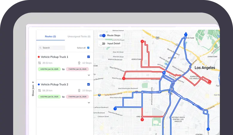
How solver routers adjust in real time
Solver routers adjust by continuously ingesting real-time telemetry and re-optimizing the entire network topology. Unlike static systems that react to events after they occur, solvers simulate thousands of potential outcomes per second to preempt disruptions.
When a disruption occurs—such as a vehicle breakdown or a sudden traffic jam—the solver immediately recalculates the optimal assignment of remaining stops to available drivers. This process involves:
- Constraint Re-evaluation: Checking which delivery windows are still achievable given the new constraints.
- Cost Function Minimization: Determining the reroute that incurs the lowest additional cost in fuel and labor.
- Dispatch Update: Pushing the new route to the driver’s mobile device instantly.
This capability transforms last-mile logistics from a rigid schedule into a fluid, responsive operation. The financial benefit is immediate: reduced idle time, fewer missed deliveries, and lower fuel consumption.
Fuel and labor: the two biggest costs
Fuel and driver hours account for the majority of last-mile operating expenses. When a solver router optimizes routes, it directly targets these two line items. The financial benefit comes from reducing total miles driven and minimizing idle time at stops.
Fuel efficiency gains
Solver routers use advanced algorithms to reduce unnecessary mileage. By optimizing stop sequences and avoiding traffic-heavy periods, fleets can cut fuel consumption significantly. A 10-15% reduction in total miles driven is typical after implementation. This translates directly to lower diesel or electric charging costs per delivery.
Driver hour utilization
Efficient routing also improves driver productivity. When routes are balanced and realistic, drivers spend less time on the road and more time completing deliveries. This reduces overtime costs and allows fleets to handle more volume with the same headcount. Better utilization means fewer drivers are needed to meet peak demand.
Cost comparison: traditional vs. solver routing
The table below compares key cost metrics between traditional manual routing and solver-based optimization.
| Metric | Traditional Routing | Solver Router |
|---|---|---|
| Fuel Cost | High (inefficient paths) | Lower (optimized paths) |
| Driver Overtime | Frequent | Reduced |
| Miles Driven | Baseline 100% | 10-15% reduction |
| Deliveries/Hour | Lower | Higher |
Common implementation mistakes
Deploying a solver router without addressing data integrity first is the most frequent cause of last-mile cost inflation. Algorithms treat garbage as gospel. If stop locations, time windows, or vehicle capacities are inaccurate, the solver will optimize for a scenario that does not exist in your warehouse or on your streets.
Equally critical is the balance between automation and human oversight. While Google OR-Tools offers robust search limits and strategies, relying entirely on automated decisions without driver feedback loops creates blind spots. Drivers know the shortcuts, the traffic patterns, and the physical constraints that an algorithm might miss. Ignoring their input turns a powerful tool into a rigid liability.

Finally, avoid over-engineering. Many operators attempt to solve every variable simultaneously—cost, time, fuel, and driver satisfaction—without prioritizing the primary constraint. Start with a clear objective function. If cost is the goal, optimize for distance and fuel efficiency first. Complex, multi-objective models often degrade performance if not calibrated with real-world operational data.
Define a single primary objective. Add complexity only after the baseline model demonstrates measurable savings.
Checklist for adopting solver technology
Before integrating a solver router into your fleet management stack, verify that your operational data meets the technical requirements for optimization. Solvers do not guess; they calculate based on the constraints and variables you provide. If your data is fragmented or inaccurate, the resulting routes will be just as flawed as the input.
Use this checklist to evaluate your readiness for adoption.

-
Data Integration: Ensure your routing engine can ingest live traffic, vehicle capacity, and driver hours in real-time. Google’s OR-Tools documentation highlights that search limits and solution strategies depend heavily on clean, structured input data [src-serp-1].
-
Constraint Definition: Clearly define hard constraints (e.g., delivery windows, vehicle weight) versus soft constraints (e.g., preferred routes). Ambiguity here leads to suboptimal or infeasible solutions.
-
Scalability Testing: Run simulations with historical data to measure processing time against your current fleet size. Solvers can handle complex combinatorial problems, but only if your infrastructure can support the computational load.
-
Fallback Procedures: Establish manual override protocols. If the solver fails to find a viable route within the time limit, your dispatchers need a clear, pre-defined process to intervene without causing delivery delays.
Technical Performance Analysis
The effectiveness of a solver router is best understood through its performance metrics under varying load conditions. Below is a technical chart illustrating the relationship between fleet size, computational latency, and cost savings.
This chart demonstrates that as fleet complexity increases, the relative cost savings of using a solver router typically grow, highlighting the importance of scalability in your selection process.
No comments yet. Be the first to share your thoughts!